Tony Cassandra
St. Edwards University
Austin, TX

A Simpler Model - Markov Decision Processes (MDP)

A discrete model for decision making under uncertainty.

States - the world is divided up into a finite set of possible states
Actions - there is a finite set of possible actions available
State Transition Function - this captures the relationship between the actions and the states. It gives a probabilistic relationship about how the state of the world can be changed by executing the various actions.
Cost/Reward Function - which gives relative measures of the desirability of various states, actions and/or combinations of the two. This is what determines the metrics to use for comparing behavioral strategies.

MDPs More Formally

S = set of states
A = set of actions
T( s, a, s' ) : S x A x S -> RealNumber = Pr( s' | s, a )
R( s, a ) : S x A -> RealNumber

MDP Example

Suppose we have a distributed agent system, where each agent has some individual responsibility. Further, the network that the host computing nodes uses is not terribly reliable.

The state is whether or not the agent is executing:

S = { OK, DOWN }

The actions can be to do nothing (just ping the agent), take active measures to find out the agent's state (costly) or give up on the agent and relocate it to a different machine.

A = { NO-OP, ACTIVE-QUERY, RELOCATE }

The state transition functions:

T( StartState, NO-OP, EndState )
	EndState
StartState	OK	DOWN
OK	0.98	0.02
DOWN	0.00	1.00

T( StartState, ACTIVE-QUERY, EndState )
	EndState
StartState	OK	DOWN
OK	0.98	0.02
DOWN	0.00	1.00

T( StartState, RELOCATE, EndState )
	EndState
StartState	OK	DOWN
OK	1.00	0.00
DOWN	1.00	0.00

The reward function

R( Action, StartState )
	StartState
Action	OK	DOWN
NO-OP	+1	-10
ACTIVE-QUERY	-5	-5
RELOCATE	-22	-20

If the agent fails, then relocating is more certain to bring it back up, but also more costly.

We are interested in knowing what will be the best decision strategy "in the long term". i.e., If the agent is DOWN are we better off restarting or relocating?

Note that we will also assume that time is discrete.

Acting in MDPs

With such a small problem, one can imagine doing some simple calculation using the model parameters and being able to relatively easily determine the best strategy.

This is what the algorithms for finding the optimal decision strategies in MDPs do, only they can deal with the trade-offs between values and probabilities when there are thousands of states.

The algorithms for optimal decision strategies in MDP domains are well known and are efficient.

Very useful here is that it can be shown that the optimal decision depends only on the current state. We do not have to remember the history of where we have been and what we have done. This is the Markov property.

Thus, the optimal solutions can take the form of a policy that maps states to actions:

Policy : S —> A

This makes acting optimally as quick and easy as a table lookup. (once the calculations are done).

Problem: To apply this policy, you have to know the agent's state.

If you are the decision maker, located remotely, there are many things that might prohibit you from knowing whether the agent is still running. e.g.,

The network may go down somewhere, but the agent is still running.
The agent reports that it is running, when in fact, only the thread that responds to "ping" requests is actually running (I've seen this happen in distributed agent systems.)

The decision maker is now not sure what the agent's state is when you have to make decisions.

The decision maker probably has some information about the agent's state, but it may not be absolutely reliable.

POMDPs

Domains in which there is only partial information available about the current state is what led to the extension of the MDP to account for uncertainties in the decision maker's observations of the state of the world.

A POMDP extends an MDP by adding:

Observations - a finite set of observations of the state, a.k.a., responses, diagnoses, perceptions, views, etc.
Observation Function - captures the relationship between the state and the observations (and can be action dependent).

Note that the set of observations and the set of states are not the same. What you observe from a state is not the same as the state itself.

These observations can be used to model:

perceptual aliasing (many states give the same observation)
noisy or faulty sensors
or both, noisy aliased states

It turns out that these are theoretically all equivalent, but from a modeling perspective this helps to think about characteristics of problems.

POMDPs More Formally

S = set of states
A = set of actions
Z = set of observations
T( s, a, s' ) : S x A x S —> RealNumber = Pr( s' | s, a )
O( s, a, z ) : S x A x Z —> RealNumber = Pr( z | s, a )
R( a, s ) : S x A —> RealNumber

POMDP Example

The observations is what gets returned from either the no-op (ping) or active query actions:

Z = { ping-ok, ping-timeout, active-ok, active-down }

The observation probability functions:

O( NO-OP, State, Observation )
	Observation
State	ping-ok	active-ok	ping-timeout	active-down
OK	0.970	0.000	0.030	0.000
DOWN	0.025	0.000	0.975	0.000

O( ACTIVE_QUERY, State, Observation )
	Observation
State	ping-ok	active-ok	ping-timeout	active-down
OK	0.000	0.999	0.000	0.001
DOWN	0.000	0.010	0.000	0.990

O( RELOCATE, State, Observation )
	Observation
State	ping-ok	active-ok	ping-timeout	active-down
OK	0.250	0.250	0.250	0.250
DOWN	0.250	0.250	0.250	0.250

Raw Example POMDP Parameters

Acting in POMDPs

With the MDPs, it did not require remembering the history to act optimally: the optimal policy had the Markov property.

With POMDPs, this is not the case: the optimal thing to do now, may depend on the entire history of actions taken and observations made.

Remembering entire histories can be cumbersome, and specifying policies over the space of histories is no fun either.

Fortunately, a better way was found.

Belief States

We have a set of states, but we can never be certain where we are.

A way to model this situation is to use probabilities, i.e.,

Pr( s = OK ) = 0.75
Pr( s = DOWN ) = 0.25

(where s = state at time 't')

This captures the relative likelihood of being in these two possible states.

Generalizing, a "belief state" is a probability distribution over all possible model states.

If we are given a belief state for time 't', and we perform an action 'a' and get observation 'z' we can compute a new belief state for time 't+1' by simply applying Bayes' Rule and using the model parameters.

A key result is that if you maintain a probability distribution over model states and update it in this fashion, then it can be show that using this belief state gives you just as much information as the entire action-observation history would. (It is a sufficient statistic for the history [ Astrom, Striebel, 1965 ]).

In the original view of the POMDP, since you had to keep track of the entire history to act optimally, these solutions are non-Markovian. However, the optimal POMDP solution is Markovian over the belief state space.

In fact, using the belief space as our set of states, we can use the transition and observation probabilities to create a completely observable, regular MDP that is equivalent t the original POMDP. Major caveat: This is a continuous state space MDP, not a discrete one.

Policies for POMDPs

In general, while an MDP policy mapped states to actions, an optimal POMDP policy maps belief states to actions.

Main problem is that the space of all belief states is continuous.

This is a big part of why these problems are hard to solve.

Nevertheless, there are algorithms that can work in the space and yield optimal solutions: though they are somewhat complex and computationally inefficient.

Once the policy has been computed (either optimal or otherwise), using the solution is relatively simple and computationally easy.

The way in which one would use a computed policy is to start with some a priori belief about where you are in the world. The continually:

Use the policy to select action for current belief state;
Execute the action;
Receive an observation;
Update the belief state using current belief, action and observation; then
Repeat.

For the example we have been showing, this is the optimal policy:

Pr( State=OK )	Action
`0.000 to 0.237`	RELOCATE
`0.237 to 0.485`	ACTIVE
`0.485 to 0.493`	ACTIVE
`0.493 to 0.713`	NO-OP
`0.713 to 0.928`	NO-OP
`0.928 to 0.989`	NO-OP
`0.989 to 1.000`	NO-OP

Note that because there are only two states, we can represent a belief state with a single value.

Thus, acting in a POMDP with a precomputed policy winds up being not much more than a table lookup and an application of Bayes Rule.

Policy Graphs

Here is an alternate form of a policy for acting in a POMDP. Instead of tracking the belief state and using a table lookup, we define a graph.

Construct a finite state controller such that each node of the graph has an associated action, and there is one arc out of the node going to some other node for each observation that is possible.

For our example, here is a candidate finite state controller, which is sometimes called a "policy graph":

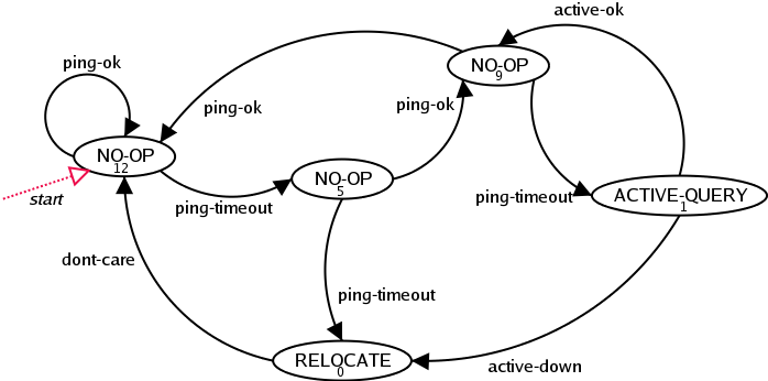
To use this, we pick a starting node, then:

Execute the action that the current node tells us to;
Receive the resulting observation from the world;
Transition to the next node based on the observation; then
Repeat.

This can certainly serve as a controller for the POMDP, but the question would be how well can it control the POMDP.

It turns out that if you have a POMDP model, a policy graph and know the starting (a priori) belief state, then you can evaluate the policy graph and determine exactly how well it will do in terms of the expected reward.

You take the POMDP model and the policy graph, set up a system of equations, solve the equations, then take the dot-product of the result vector of values with the a priori belief state and you get a single number.

Do this same thing for a different policy graph and you will get another number. The policy graph with the larger number is the better one.

One way to try to derive solutions to POMDPs is to search over the space of these policy graphs [ Hansen, UAI-98 ; Meuleau, et al, UAI-99 ]

The search space is enormous, especially if you do not know how many node you will need in the policy graph.

Value Functions

That example policy graph will actually yield the optimal behavior for this POMDP.

However, it was not found by searching in the space of policy graphs: it was derived after computing the optimal value function.

Assuming you knew how to behave optimally, you could compute exactly how much expected reward you could achieve from any given belief state (by just cranking through the formulas and tracing all possible action-observation sequences.)

For each belief state you get a single expected value, which if done for all belief states, would yield a value function defined over the belief space.

Thus, an alternative to searching over the space of policy graphs is to search over the space of value functions. [ Hauskrecht, JAIR 2000 ; Littman, et al, ML 1995; Parr and Russell, IJCAI 1995 ]

The exact POMDP algorithms do not so much as search the space of value functions, but construct the value function. [ Sondik 1971, Cheng 1988, Littman 1996; Cassandra 1998; Kaelbling 1998; Zhang 1998 ]

For this example, we used an exact algorithm to compute the optimal value function, which yielded:

Some important points about the process of constructing this value function:

It is always piecewise linear and convex, consisting of the upper surface of a number of hyper-planes.
Each linear segment is representing a value directly associated with a single action. For this example:
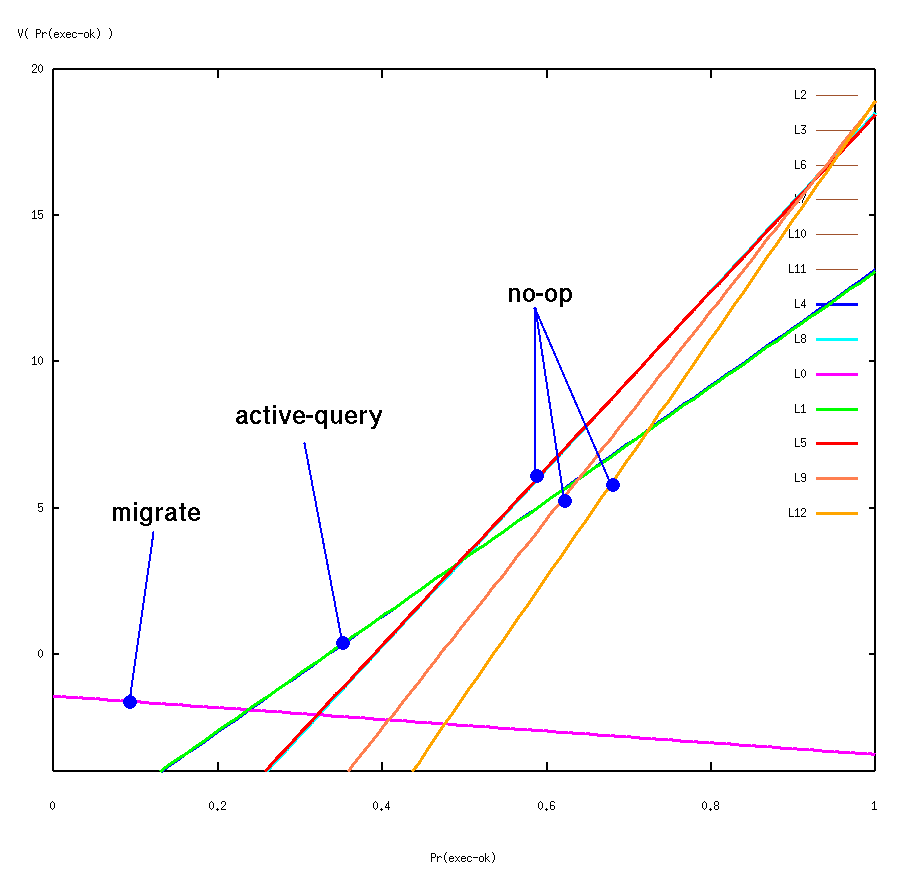
The intersections of the hyper-planes partition the belief space into a finite number of equivalence classes. i.e., all belief states where the optimal action is the same and whose value lies along the same linear slope.

Belief State Dynamics

Without going into too many details, this particular problem's optimal value function has a very nice property (called finite transience, [ Sondik 1971, Cassandra 1998 ]).

The property is derived from the POMDP model parameters, and works out that:

For all belief partitions, B_i, if for any b in B_i, T(b,a,z) is in B_j for any action 'a' and observation 'z', then for all other b' in B_i, T(b',a,z) is also in B_j.

i.e., all belief states in the same partition get transformed (the belief update equation) to exactly the same partition for a given action and observation.

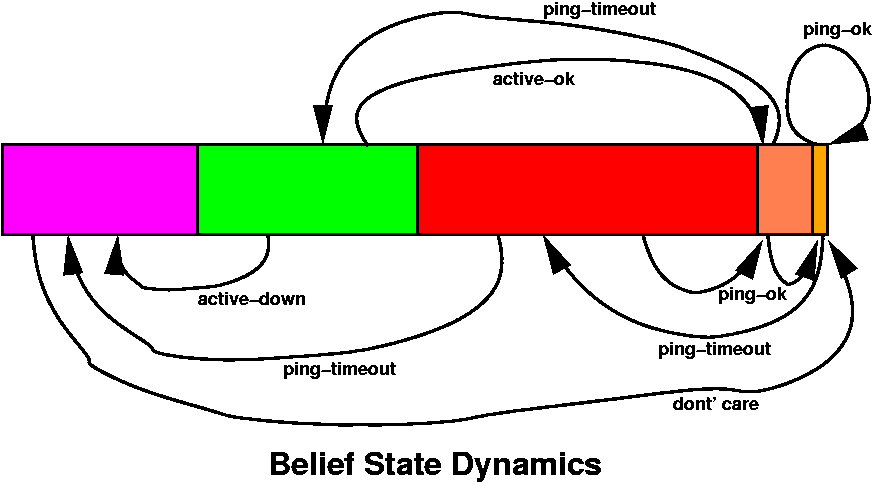
Note: Not all optimal POMDP policies have this property.

It is this convenient property that allows us to convert the value function into a policy graph.

Each belief equivalence class becomes a node in the graph, and the belief dynamics define the edges of the graph.

Truth in Advertising

What we have been showing is actually a slight simplification of the optimal policy graph. The full policy graph looks like this:

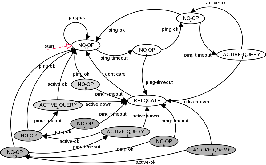
Comments on this full policy graph:

If we always start with the initial belief that the agent is certain to be in the OK state, then none of the shaded nodes will ever be needed. i.e., no sequence of actions and observations (following this policy) can transform the initial belief Pr(state=OK) = 1.0 into a belief state covered by the shaded nodes.
The six darkest shaded nodes (2, 3, 6, 7, 10, 11) cover a belief partition that is exceedingly small (less than 1E-7).

Searching in Belief Space

Just to briefly mention another possible technique for solving POMDPs:

If you know the starting (a priori) belief state and have the POMDP model parameters, you could compute all the possible future belief states by just trying all combinations of action-observations histories.

Additionally, as you do this, you could compute an expected value using the model rewards parameters, and take the maximum actions at each step in the history.

This too is a very large search space.

This belief space search represents a "forward" calculation of expected values.

The algorithms for computing the optimal value functions use dynamic programming and thus represent a "backward" calculation of the expected values.

Recent Stuff: Spatial Navigation

I have recently gotten involved in helping Brian Stankiewicz in the psychology department here at UT. Brian is using POMDP models to help study human spatial navigation.

Brian does not care how efficient the algorithms are, he just wants to have a benchmark against which to compare human performance.

See how the optimal behavior degrades versus the human behavior as the complexity of the environment is increased. Then exploring the reasons why human performance falls off more quickly that the optimal.

Brian's domains:

Rectilinear hallways,
Discretized locations,
Limited (4) observer orientations,
Limited observations (views down hallways),
Goal location.

The interesting things about this were:

Brian had developed his own search algorithm for solving this, which essentially was a search in belief space;
Brian could optimally solve problems in his domain that had hundreds of states.

I had believed that I had the world's fastest code for computing optimal POMDP solutions, but my code could not solve these problems in anywhere near the time Brian was doing it (if it might have been able to solve them at all).

How could this be?

It turns out that Brian's domains have a lot of structure that can be exploited. Brian's algorithms were exploiting it, while my algorithms were not.

Once I realized what the structure was, I tweaked my code to exploit it, and could then solve his problems in a matter of seconds. So there.

Converting a Hard POMDP to an Easy MDP

Brian's domains had deterministic actions and deterministic observations. What made it a POMDP was that certain locations were perceptually aliased.

Further, Brian always assumed that the person started in the same confused state (they were equally likely to be started anywhere in the domain).

These dynamics gave the domains the property that there were only a small, finite number of possible belief states that could ever be visited.

In general, there are only a polynomial number of belief states in domains such as this (polynomial in the size of the problem).

Briefly:

The a priori belief is the uniform distribution over all states.
After the first observation, we can eliminate (set the probability to zero) any state from which this view is not possible (observations are not unique, but are deterministic.)
The resulting belief state is again a uniform distribution, though this time possibly over a smaller set of states.
After each observation and belief update, we are always left with a uniform distribution.
Instead of using a vector of probabilities to represent the belief state, we could simply use a set of states (all those whose probability is not zero).
This set of states is guaranteed to never grow larger, due to the deterministic state transitions and observations.
Since there is only a finite, polynomial number of belief states, and since we can derive a completely observable MDP over belief states, we can convert the original problem into a finite state space MDP.
Thus we are solving a polynomial-sized problem, using a polynomial time algorithm (completely observable MDP solutions are efficient.)

The bottom line here is though the general case of a POMDP is computationally hard (PSPACE-complete or even undecidable), classes of problems have exploitable structure that can reduce the complexity.

Additional Recent Stuff: Distributed Agents

Applying POMDP models to DARPA's Ultralog/Cougaar program.

Distributed agent system for military logistics.

Military is concerned about the robustness of the system in the face of deliberate and unintentional failures.

Large distributed agent communities are most certainly only partially observable.

Complete model and optimal solution of this problem is not the goal (nor would it be feasible).

Modeling smaller, specific portions and combining heuristic methods is the goal.

Model and belief update alone provides a great improvement

Previous handling of robustness issues were many ad hoc solutions that often conflicted. Using the POMDP model to unify the view of the problem and add clarity the problem space.

Some interesting semantic and cultural problems have cropped up while trying to move to this model.

POMDP Model Problems

For non-trivial modeling, the state/action/observation spaces quickly grow, This is a result of requiring a complete enumeration of all possible states (aka, a flat state space)

Model the problem hierarchically [ TBR: Pineau and Thrun, 2000 ; Theocharous and Mahadevan, 2002, Theocharous 2002 ]
Use a factored state space representation [ Boutilier and Poole, AAAI 1996 ] [ TBR: Hansen and Feng, 2000 ; Guestrin, et all, 2001 ]

Discrete, uniform time elapsing between each action-observation pair is not always a good assumption (especially in Ultralog/Cougaar domain).

Assumption that the model will not change over time (non-stationary process) does not always apply (especially in Ultralog/Cougaar domain).

Assumption that you know the full domain dynamics (i.e., the model) [ Chrisman, AAAI 1992 ] [ TBR: Nikovski 1998 ]

Assumption that the POMDP model is completely accurate.

Conclusions

Regardless of the efficiency of the representation and solution techniques, viewing the problem as a POMDP allows a much clearer understanding of the problem domain.

Even when optimal solution is not feasible, modeling the domain using a POMDP and computing the efficient belief state update tracking is very useful.

Understanding the domain dynamics, properties and optimal solution techniques only helps to gain insight into deriving the next generation algorithms and representations.

Future Work

More work needs to be done exploring combinations of policy, value and belief space search.

More work on hierarchical and factor state representations.

There is a large space of possible heuristic solutions, but more work needs to be done in exploiting domain structure.

Exploration of alternate models: [e.g., PSRs: Singh, Littman, Sutton and Stone]

POMDPs: Who Needs them?